A goodness-of-fit test, introduced by Karl Pearson in 1900, that is popular because of its simplicity. Let O denote the observed frequency of an outcome in a sample and let E denote the corresponding expected frequency under some model. The test statistic is X², defined by where the summation is over all the outcomes whose frequencies are being compared, and r, the Pearson residual, is defined byIt is important to note that the comparison involves frequencies and not proportions.

If there are m observed frequencies, and p parameters have been estimated using these frequencies, then, if the model is correct, the observed value of X² will approximate an observation from a chi-squared distribution with (m−p−1) degrees of freedom. In the case of a continuous random variable, the frequencies will refer to ranges of values. For other random variables it is usual to combine together neighbouring rare values into a single category, since the chi-squared approximation fails if there are too many small expected frequencies.

As an example, suppose it is hypothesized that a type of sweet pea occurs in shades of white, red, pink, and blue, with proportions ¼, p, (¾−3p), and 2p, respectively. A random sample of 120 seeds is sown. All germinate with 20 having white flowers, 10 having red flowers, 40 pink, and 50 blue. The question is whether these results are consistent with the hypothesis. In this case the maximum likelihood estimate of p is 0.15, so the expected frequencies are 30, 18, 36, and 36. ThusThere are 4−1−1=2 degrees of freedom. Since 12.8 is a very large value (compared with the percentage points (Appendix VIII) of a -distribution), the hypothesis can confidently be rejected.

One situation in which the use of the chi-squared test is frequently encountered is as a test for independence in a J×K contingency table that cross-classifies the variables A and B. Let the observed frequency of data belonging to category j of variable A and to category k of variable B be f_jk. Write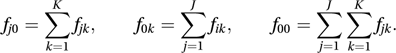Then, according to the null hypothesis of independence, the expected frequency e_jk is given byand the test statistic X² is given by 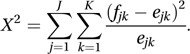If the null hypothesis of independence is correct, then the distribution of X² can be approximated by a chi-squared distribution with (J−1)(K−1) degrees of freedom. In the special case where J=K=2 (a two-by-two table), the chi-squared approximation is improved by using the Yates-corrected chi-squared test (see two-by-two table).

In 1946 Cramér suggested that a measure of association could be based on the value of X². This is Cramér's V, given by where M is the smaller of J−1 and K−1.