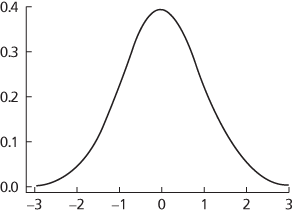
The type of statistical distribution followed by, for example, the same measurement taken several times, where the variation of a quantity (x) about its mean value (μ) is entirely random. A normal distribution has the probability density function
where σ is known as the standard deviation. The distribution is written N(μ,σ2). The graph of f(x) is bell-shaped and symmetrical about x=μ. The standard normal distribution has μ=0 and σ2=1. x can be standardized by letting z=(x − μ)/σ. The values zα, for which the area under the curve from −∞ to zα is α, are tabulated; i.e. z is such that
Hence
can be found.
The continuous probability distribution with probability density function f given by
denoted by N(µ, σ2). It has mean µ and variance σ2. The distribution is widely used in statistics because many experiments produce data that are approximately normally distributed; the sum of random variables from non-normal distributions is approximately normally distributed (see Central Limit Theorem), and it is the limiting distribution of distributions such as the binomial, Poisson, and chi-squared distributions. It is called the standard normal distribution when µ = 0 and σ2 = 1.

Density function of standard normal
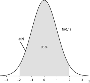
If X has the distribution N(µ, σ2) and Z = (X−µ)/σ, then Z has the distribution N(0,1). The diagram shows the graph of the probability density function of N(0,1).
The table gives, for each value z, the percentage of observations which exceed z, for the standard normal distribution N(0,1). Thus the values are to be used for one-tailed tests. Interpolation may be used for values of z not included.

P(Z≥z) as percentages
The distribution of a random variable X for which the probability density function f is given by
 The parameters μ and σ2 are, respectively, the mean and variance of the distribution. The distribution is denoted by N(μ, σ2). If the random variable X has such a distribution, then this is denoted by X ∼ N(μ, σ2) and the random variable may be referred to as a normal variable.
The graph of f(x) approaches the x-axis extremely quickly, and is effectively zero if |x−μ|>3σ (hence the three-sigma rule). In fact, P(|X−μ| < 2σ)≈95.5% and P(|X−μ|<3σ)≈99.7%. The first derivation of the form of f is believed to be that of de Moivre in 1733. The description ‘normal distribution’ was used by Galton in 1889, whereas ‘Gaussian distribution’ was used by Karl Pearson in 1905.
The normal distribution is the basis of a large proportion of statistical analysis. Its importance and ubiquity are largely a consequence of the Central Limit Theorem, which implies that averaging almost always leads to a bell-shaped distribution (hence the name ‘normal’). See bell-curve.
The standard normal distribution has mean 0 and variance 1. A random variable with this distribution is a standard normal variable. It is often denoted by Z and we write Z ∼ N(0, 1). Its probability density function is usually denoted by ϕ and is given by
 If X has a general normal distribution N(μ, σ2) then Z, defined by the standardizing transformation
 has a standard normal distribution. It follows that the graph of the probability density function of X is obtained from the corresponding graph for Z by a stretch parallel to the z-axis, with centre at the origin and scale-factor σ, followed by a translation along the z-axis by μ.
The cumulative distribution function of Z is usually denoted by Φ and tables of values of Φ(z) are commonly available (see Appendix v; see also Appendix iv). These tables usually give Φ(z) only for z>0, since values for negative values of z can be found using

The tables can be used to find cumulative probabilities for X ∼ N(μ, σ2) via the standardizing transformation given above, since, for example,
 As an example, if X ∼ N(7, 25) then the probability of X taking a value between 5 and 10 is given by
 The normal distribution plays a central part in the theory of errors that was developed by Gauss. In the theory of errors, the error function (erf) is defined by
An important property of the normal distribution is that any linear combination of independent normal variables is normal: if and are independent, and a and b are constants, then

with the obvious generalization to n independent normal variables. Many distributions can be approximated by a normal distribution for suitably large values of the relevant parameters. See also binomial distribution; chi-squared distribution; Poisson distribution; t-distribution.

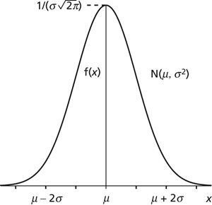
Normal distribution. The diagram illustrates the probability density function of a normal random variable X having expected value μ and variance σ2. The distribution has mean, median, and mode at x=μ, where the density function has value 1/(σ√2π). Note that almost all the distribution (99.7%) lies within 3σ of the central value.

Standard normal distribution. The distribution is centred on 0, with 99.7% falling between −3 and 3 and 95% falling between −1.96 and 1.96.
A statistical probability density function that is represented as a symmetrically bell-shaped graph in which data is symmetrical with a mean, μ, and standard deviation, σ. It has a near-zero start and rises in a smooth-bell shaped peak of probability in the centre and descends to near-zero at the end. It was also known as the Gaussian distribution, named after German mathematician Karl Friedrich Gauss (1777–1855) and was first derived by French mathematician Abraham de Moivre (1667–1754). The probability density function is:
An important probability distribution for data in the form of continuous measurements. The frequency function is given by
The distribution is symmetric about the mean, μ, and its variance is σ2. The range of x is infinite (–∞, ∞). Many sampling distributions tend to the normal form as the sample size tends to infinity.
See Gaussian distribution.
In statistics, a continuous probability distribution which is asymptotic and symmetrically bell-shaped about the mean. The normal distribution is widely applied in statistics to model continuous variation. The two parameters of the distribution are the mean and variance. See also central limit theorem.
A continuous distribution of a random variable described by a probability density function of the form
The normal distribution has mean μ, variance σ2, and is symmetric about the mean. The standard normal distribution is defined as the normal distribution with zero mean and unit variance; normal distributions with arbitrary mean and variance form a location-scale family. The normal distribution plays an important role in statistical inference due to the Central Limit Theorems.
- phenolphthalein test
- phenols
- phenol–formaldehyde resin
- phenome
- phenomena bene fundata
- phenomenalism
- phenomenological relations
- phenomenology
- phenomenon
- phenomenon instance
- phenon
- phenotype
- phenotypic plasticity
- phenoxy resins
- phenylalanine
- phenylamine
- phenylammonium ion
- phenylenediamine
- phenylethene
- phenyl group
- phenylhydrazine
- phenylhydrazones
- phenylketonuria
- phenylmethanol
- phenylmethylamine